HOUDINI - FLIP SIMULATION PART 2
(FLIP TANK)
INTRODUCTION
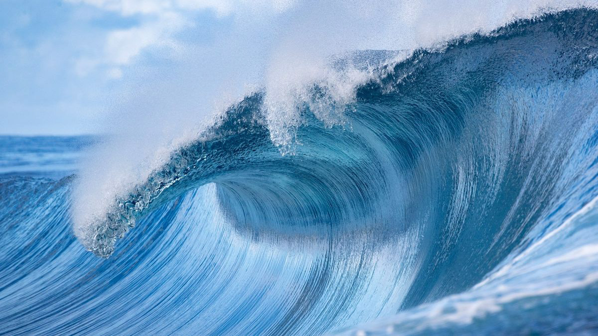
FLIP Tank simulation is a method we use to simulate a large body of water such as a river or an ocean. We can use external influences to create disturbance on the water surface (like ocean waves and ripples) or to make it flow in a specified direction (like a river). We are going to dive straight into setting up a FLIP tank inside Houdini in the next section.
FLIP TANK SETUP
We will start by creating an empty geometry node and name it as "source". Then we will enter into it's SOP level. The first thing we want to create is an 'ocean source' node. This is where our ocean flip particles will be sourced from. It will create an empty bounding box for us.

Select the node and change the 'initialize' parameter from 'wave tank' to 'flat tank'. This generates some points inside the box for us. Add a null to the output and name it "source_out".

We can use the 'Water Level' parameter to raise or lower the water level. Next, let us go back to the object level and create a new 'dopnet' node and enter into it's SOP level. Let us create our basic flip setup like we learnt in the basic flip module. We should have something like below:

If you recall in the last module, we need points to serve as the source of the flip particles. The idea is the same with flip tank. Since we have already generated some points with the ocean source node, we can easily convert these points into flip particles.
So we will change the input type on the flip object node to 'particle field', and then reference-in the "source_out" null node into the SOP path field. We will also use relative referencing to match the size and center of the flip solver bounding box to the size and center of our ocean source bounding box. We should also link the particle separation of the flip object node to the particle separation of the ocean source node for consistency. Also do not forget to check on 'closed boundaries' so that the bounding box acts as a collision container for the flip particles.. Now, the ocean source points should now be converted into flip particles.

ADDING COLLISION
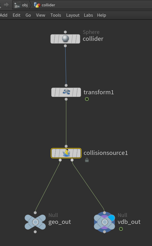
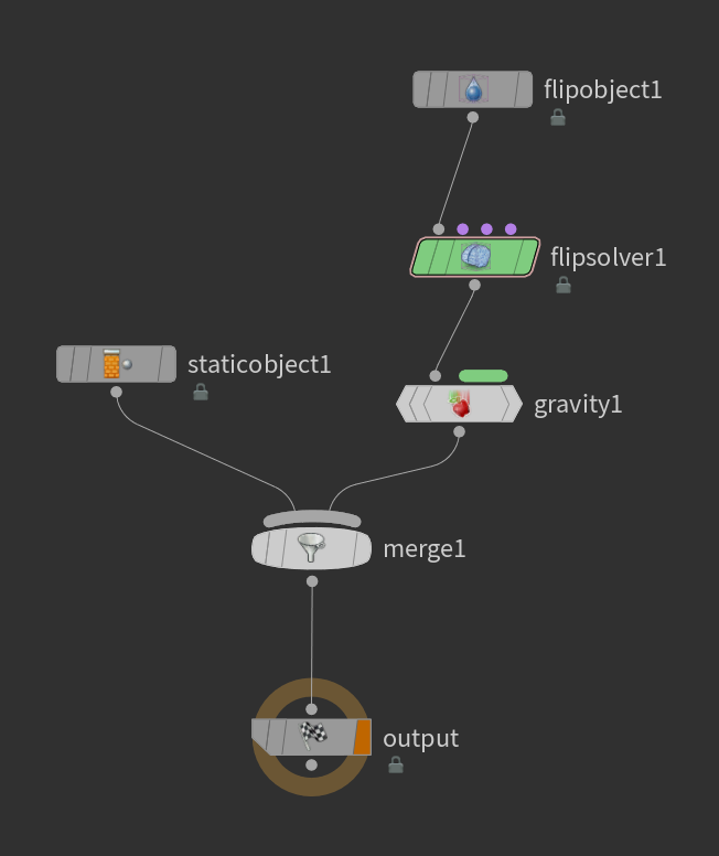
The next thing is to add a collider geometry. We will follow the same approach we learnt in the last module to set up a collision geometry. For this example, we created a simple sphere, scaled it up, and animated it to fall into the flip tank. We then added a collision source node and referenced it into our flip simulation via the 'static object' node. When we play the simulation, the sphere now collides with the flip particles, creating a splash.
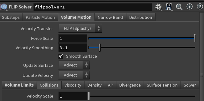
Under the collision flip solver volume motion's collision subtab, we can increase the 'velocity scale' parameter to increase the splash effect of the simulation. However be careful because doing this will globally affect every colliders present in the scene and may give undesirable results. So instead, we will need to create different solvers for each colliders we want to have more splash and use a merge node to combine them back to the flip setup. We will dive more into this in later sections.
NARROW BANDING
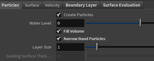
Narrow banding is a method used in flip tank simulation. In order to see and understand how this work, let us start by first enabling 'narrow band particles' on the ocean source node.
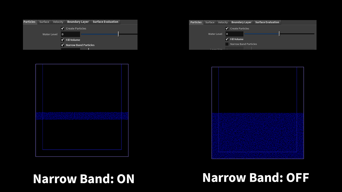
As we can see from above, enabling narrow band particles trimmed the volume of our ocean body into a sort of 'slice'. The thickness of this slice can be increased or decrease via the 'layer size' setting under the particles subtab of the ocean source node. Also, it is a good idea to always keep the water level at 0 to avoid any issues.
If we play the simulation, these narrow band particles are going to fall straight down as if there is no volume below them to retain them.
In order to retain the volume of our ocean, we will need to change the input type on the flip object node from 'particle field' to 'narrow band'. Next, we will reference-in the ocean source null output into the 'surface volume' field. Lastly, let us go to the narrow band tab of the flip solver and enable 'particle narrow band'.


If we play the simulation again now, the volume of our ocean is retained without falling like before. We will notice that the level of the ocean dipped a bit but the overall volume is still retained.
In real practice, the idea of using narrow band is to be able to simulate a large ocean body. However, it would be computationally costly to simulate the entire ocean all at once. So, to facilitate a smooth workflow, we can use the bounding box and narrow banding to mask out the portion of the large ocean body that we wish to simulate. Later on, we will learn the method for integrating our flip simulation with an infinite ocean body.
In real practice, the idea of using narrow band is to be able to simulate a large ocean body. However, it would be computationally costly to simulate the entire ocean all at once. So, to facilitate a smooth workflow, we can use the bounding box and narrow banding to mask out the portion of the large ocean body that we wish to simulate. Later on, we will learn the method for integrating our flip simulation with an infinite ocean body.
The advantages of using narrow band are as follows:
1. If we allocate say 10 GB RAM to evaluate say a total of 1 million flip particles in a flip tank and we enable narrow banding, this will slice up the ocean body into a narrow band which will now contain far lesser particles than the total flip particles in the ocean. That means we will now have more room for resolution in the same amount of RAM in order to get finer details in our simulation.
2. When we cache out the simulation, it will not evaluate any ocean particles that isn't present in the narrow band, so the cache size will be lesser.
Unfortunately, narrow banding does not make our simulation any faster.
FIXING REFLECTION ON BOUNDING BOX
Currently, our simulation so far looks like it is confined within a box, so when we simulate, they collide with the bounding box and reflect back into the flip tank. We can set it up such that it does not feel like it's confined in a box.
To do this, go to the volume subtab of the flip solver and enable 'use boundary layer'. Then reference-in the ocean source null output into the 'surface volume' path field.

Now let us understand how the boundary layer works. The boundary layer is a sort of padding around the edges of the bounding box and can be added on all three axes. In the case of simulating an ocean (or a river), we will not include the y-axis in the padding.
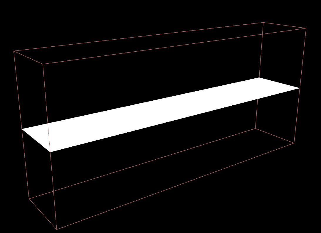
The lower padding is in the negative and the upper padding is in the positive direction. For example, if we punch in a padding of 1 on lower and upper padding of both x and z axes, we will get this result at the edges of the bounding box:
The lower padding is in the negative and the upper padding is in the positive direction. For example, if we punch in a padding of 1 on lower and upper padding of both x and z axes, we will get this result at the edges of the bounding box:


This boundary layer will eliminate any particle that leaves the bounding box and will birth (or seed-in) new particles that enters into the bounding box.
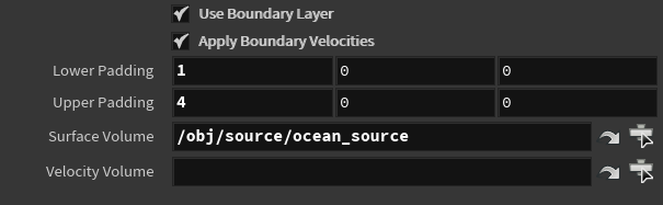
BOUNDARY VELOCITY
We can also use the 'apply boundary velocity' to introduce velocity into the flip tank at the boundaries. This is useful for simulating a river for example. If we set the lower padding on x-axis to say 1, and the upper padding on x-axis to say 4, the particles will be reseeded from the higher value boundary padding to the lower value boundary padding, and in this case, from +x axis to -x axis.

We can use a velocity volume to increase the effect of the velocity at the boundary layers by introducing an instantaneous velocity and specify it's magnitude and direction.
We will instantiate the velocity volume in the source SOP level by creating a 'volume' node. We can use relative referencing to match the size and center of this volume to the flip bounding box.
Next, we will change it's rank from 'scalar' to 'vector', since velocity is a vector quantity, and in the name field, we will type 'vel', which represents 'velocity'. We can now initialize the velocity by setting an initial value in the preferred direction.
Also turn on the 'two dimensional' so we can see it's bounding box shape and set it to ZX plane so that it aligns with the surface of the water body.
We will then connect a null output node and reference this into the 'velocity volume' path field.


If we play the simulation now, we will see that the velocity has been introduced to our flip particles in the specified direction.
****************LET'S CREATE A BEACH!!!*******************
To recap everything that we have learnt so far about flip tank, we will create a beach simulation as an exercise. The stages of this exercise are broken down below:
1. CREATE THE TERRAIN
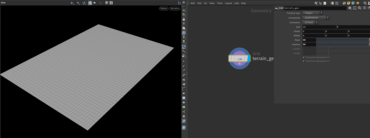
We will start this exercise by first creating the terrain on which the beach water is going to interact with. Create an empty geometry node and rename it as "terrain" and go into it's SOP level. Here we will create a grid and set it's size and also increase the number of rows and columns resolutions.
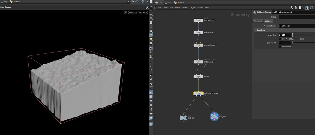
Let us add a transform node and rotate it along z-axis until it is inclined to the horizontal.
Then we will add a polyextrude node to give it some thickness since we intend to use this as a volume collider later.
Next we will use a mountain node to add some roughness to the surface of the terrain.
Finally, we will add a collision source node and connect two nulls to it's output.
We should have the following result:
2. CREATE THE OCEAN SOURCE
We will simply create the ocean source like we have learnt in the previous section. So let us proceed to the next stage.
3. CREATE THE FLIP SETUP
As usual, we will create the dopnet and create our flip tank set up like we have learnt in the previous sections. We will link the flip solver bounding box to the ocean source bounding box, and particle separations as well.
We will also resize and reposition our bounding box to where we want the beach to be. While resizing our bounding box, it is important that we size up our bounding box up to the extents where we want the flip particles to reach during the simulation. If we don't do this, during meshing, we will face an issue where the flip mesh are visibly colliding with the bounding box at the position where the bounding box stops.
Next, we will also add the terrain as a collider to our setup.
If we do everything correctly, our scene should look as follows:

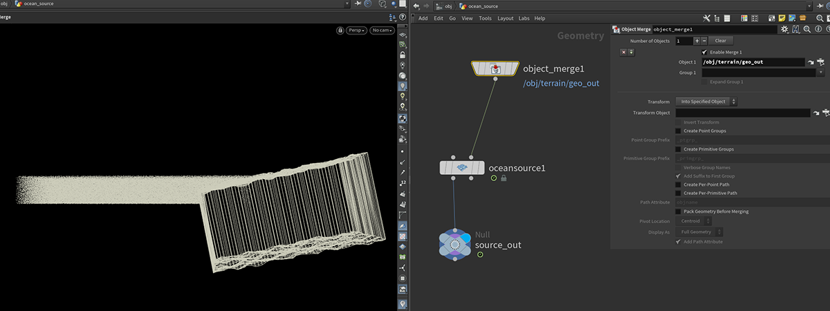
We will notice that the flip particles are inside of the terrain geometry, and if we play the simulation, we will get a weird result. To fix this issue, we need to remove those flip particles that are inside the terrain. To do this, let us go into the ocean source SOP level. Let us use an 'object merge' node to import the terrain geometry (geo null) into this SOP level. Then we will connect this node to the 'collision geometry' input of the ocean source node. This will immediately delete all the points within the collider geometry, and this in turn would be effected in the flip setup. We should also enable 'Kill Inside Collision' on the ocean source node.
Now, we've been able to trim out those confined flip particles.


Next, let us go to the particle motion tab of the flip solver and turn off 'collide with volume limits' so that the flip particles do not collide with the bounding box.

Now we are set to proceed to the next step.
4. ADDING OCEAN DISTURBANCE
Currently, our beach water looks still, so we are going to add some ocean disturbance so that the water splashes against the beach terrain. We will do this by adding ocean waves to our ocean source node.
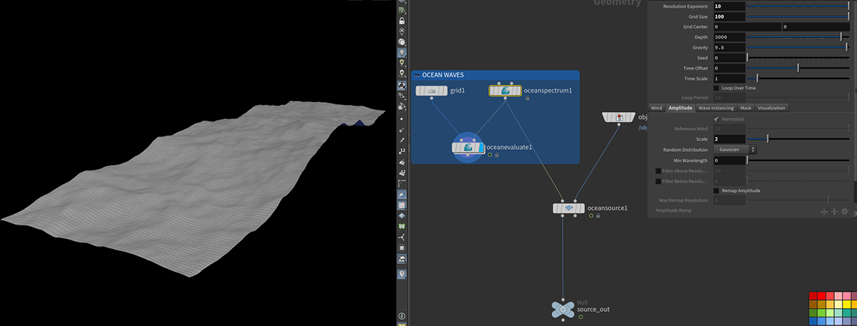
First, let us create an 'ocean spectrum' node, an 'ocean evaluate' node, and a grid geometry (for previewing the waves) and connect them as follows:
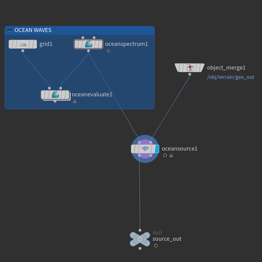
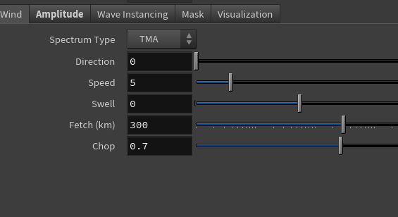
Let us also match the size of the grid to the surface of our ocean, and position it such that it lies on the surface of the ocean. If we enable the ocean evaluate, we will see that the grid now deforms. We can achieve different behaviour for the wave via the ocean spectrum node by tweaking the wind and amplitude properties of the ocean spectrum node.
But now, if we play the simulation, we don't see any waves. Let us modify our flip setup so that the waves affect our flip particles.
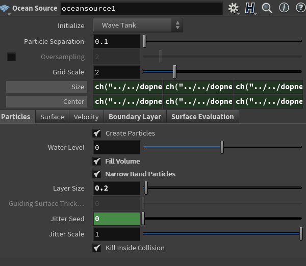
First, let us change the initialize of the ocean source node to 'wave tank'. Let us enable 'narrow band particles' and punch set layer size to 0.2, and water level to 0.
Go to the flip object and change the input type to 'narrow band', and reference-in the ocean source null output in the 'surface volume' field.
On the flip solver, enable 'particle narrow band'. In the volume limits subtab under volume motion tab, enable 'use boundary layer' and give it some padding so that the flip particles do not collide with the boundary box.
We can also turn off -z of the closed boundaries on the flip object node so that any flip particles that reaches there is killed off.
Now our simulation should work.
We can further fine tune the simulation and increase the resolution of the simulation. Once we are satisfied with the look and behaviour, we can cache out the simulation using the methods we learnt in the basic flip module.
We can further fine tune the simulation and increase the resolution of the simulation. Once we are satisfied with the look and behaviour, we can cache out the simulation using the methods we learnt in the basic flip module.
5. ADDING WHITEWATER
Now that our beach simulation is working as expected, we can add some whitewater particles to make it look nicer.
To begin, let's first enable 'vorticity' in the flip solver particle motion vorticity subtab.
To begin, let's first enable 'vorticity' in the flip solver particle motion vorticity subtab.
Next we will cache out our current beach simulation using the caching techniques we have learnt before.
Next, we will add a 'whitewater source' node and connect a null output to it, renamed "ww source". Our connections should look like below:

Now that we have created the whitewater source, we will now create the whitewater simulation. We will create a new dopnet node and name it "whitewater". Inside the SOP level, we will create the following connections:

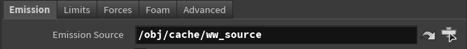
In the emission source path of the whitewater solver, we will link the null output of the whitewater source.
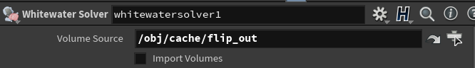
In the volume source path, we will link the null output of the flip simulation. This null output should be added to either the dopimportfield or the filecache node inside the cache SOP level.
Next, let us match the size and center of the volume limits of the whitewater to the bounding box of the flip simulation for consistency, and also turn on the 'closed boundaries' and check on all axes of the whitewater volume limits.
If we have done everything correctly, the whitewater particles should now be emitted. We can increase the base advection strength so the particles can adhere more to the flip particles and base velocity multiplier so that we get more splash effect.
Once we are happy with the results, we can now cache out the whitewater.
And if we like, we can also mesh the flip water with the particle fluid surface node.
Congratulations! You have successfully created a basic beach simulation.
